Post by Péter Rácz.
We use large cross-cultural datasets to test theories of cultural evolution. These tests face what is commonly referred to as “Galton’s problem” (see here for an elegant overview). Since cultural traits co-evolve (think historical linguistics) and are traded freely in close proximity (think Sprachbund effects), their co-variance will be partly explained by shared ancestry and geographic proximity.
This co-variance is interesting in itself, but many theories of cultural evolution seek to form generalisations about human nature. In such cases, Galton’s problem has to be accounted for. One way to do this is to use statistical methods that take co-variance into account. Another way is to use a dataset that samples societies across phylogenies and geographic regions in a representative way.
As an inconsequential exercise, I compare one such dataset, the Standard Cross-Cultural Sample (SCCS), with another, larger, non-representative dataset, the Ethnographic Atlas (EA). I access these through the D-Place database. The SCCS contains 195 societies, the EA 1290 societies. All the societies in the former are also part of the latter. This allows me to compare them directly, using the 95 cross-cultural variables in the EA.
My question is: How much variation is explained in the EA by shared ancestry and geographic proximity? How much, if any, variation do these explain in the SCCS?
In order to make a comparison, I choose the 85 categorical variables in the EA. Using an arbitrary cutoff in category size, I filtered out those variables which have a large number of small categories or where the largest category is “absent” (i.e. most societies do not really have this specific cultural practice). This left 55 variables, covering 70,100 / 120,000 observations across the 1290 societies in the EA.
I fit a binomial mixed-effects regression model (using Douglas Bates’ lme4 package in R) on each of these variables, predicting whether a society is in the largest category, and estimating an intercept, as well as a random intercept for language family and one for geographic region in D-Place. If the distribution of the largest category for the variable does not co-vary with ancestry and proximity, such a model would have very little explanatory power. If it does, the model should explain some variation in the dataset. This variation can be expressed using r², the fraction of the variation in the response variable that is explained by the model. By proxy, the r² will indicate how much the entire categorical variable co-varies with language family and region — a simple estimate of cultural co-variation.
Since the societies in the SCCS are a proper subset of the societies in the EA, I can re-fit these models on the SCCS sample only. If the SCCS sample is more representative than the EA (which has no aspirations of the sort), I expect the r² values to go down: less variation should be explained by shared ancestry and geographic proximity.
The r²-s for the 55 relevant models across the two datasets can be seen below. Bearing in mind a number of caveats (variable coding is simplistic, language family is a poor approximation of phylogeny, the SCCS sample is smaller, etc.), this can give us a sense of how much co-variation is present in the two samples.
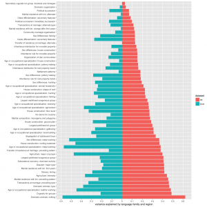
Family and region explain less variance in the SCCS than in the EA, as expected. But their effect is not negligible.
The point here is not at all to give an accurate estimation of co-variation in the SCCS or the EA. Rather, it is to encourage the use of more sophisticated statistical methods (unlike the ones used in this post) and to propagate discretion in the use of the SCCS, because human culture is more complicated than it seems.
(For data, code, and methods in graphic detail, go here.)